Reading the hidden stress field of concrete: an inverse PINN for D-regions
Our new open-access paper in Computer-Aided Civil and Infrastructure Engineering reconstructs the internal stress field of reinforced-concrete D-regions, and the load they carry, from measured strain.
Every concrete bridge has places where the textbook rules stop working. Where a pier cap receives girder reactions, where a hammerhead cantilevers from its column, where a pile cap spreads a column load into a group of piles, the assumption that plane sections remain plane no longer holds. Engineers call these discontinuity regions, or D-regions, and they are where the flow of force is most complex and where much of the reinforcement detailing effort in a bridge goes.
Our new paper, now published open access in Computer-Aided Civil and Infrastructure Engineering, asks a question about these regions that design tools are not built to answer:
Given a D-region that already exists and has sensors on it, what is the stress field inside it right now, and what load is it carrying?
- Paper: doi.org/10.1016/j.cacaie.2026.100192
- Authors: Sandesh Lamsal and Rubi Bhandari
- Access: open access, Creative Commons Attribution 4.0
Why the question matters
The United States has 623,218 highway bridges. About 45% have exceeded their planned 50-year design lives, and the rehabilitation need is estimated at $191.3 billion, according to the ASCE 2025 Infrastructure Report Card.
For an ageing structure, the useful question is rarely “what should we build?” It is “what is this member doing today, and how much reserve does it have?” That is a question of assessment, and for D-regions it is a hard one. A conventional finite-element analysis is a forward calculation: you supply the loads and boundary conditions, and it returns the stresses. In an assessment the loads are exactly what is uncertain. What an engineer has instead is partial evidence: a member standing in equilibrium, and a limited set of sensors recording its strain.
Strain sensing is becoming practical on real structures, from strain gauges to distributed fibre-optic sensing and digital image correlation. The missing piece is a rigorous way to turn those scattered measurements into the full internal stress field that a structural check actually needs.
What we built
The physics we reconstruct is the Compatible Stress Field Method (CSFM) of Kaufmann and co-workers, a code-oriented method that is already used in commercial design software. It combines a continuous stress field with kinematic compatibility and realistic material laws, including the compression softening of cracked concrete. It delivers the complete stress field of a D-region instead of a handful of strut and tie forces.
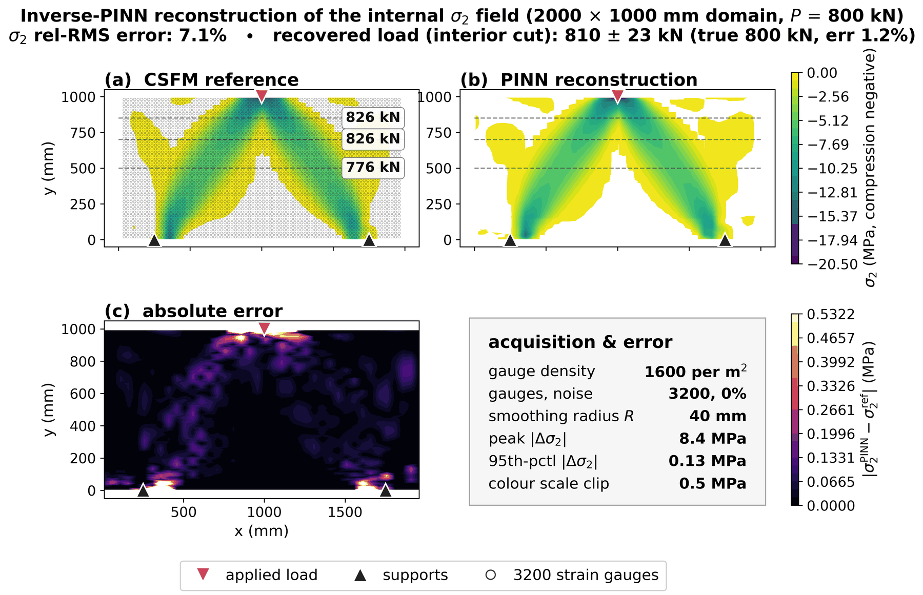
We posed the recovery of that field as an inverse problem and solved it with a physics-informed neural network (PINN):
- Two coupled networks. One network represents the strain field directly, so the measurements anchor it cleanly. A second represents the displacement field and enforces kinematic compatibility between the two.
- The CSFM built in. The cracked-membrane constitutive law, including compression softening, is embedded as a differentiable map. Every reconstructed field is a CSFM stress field by construction. The port reproduces the reference solver’s element stresses to within 0.6 to 2.7%.
- No loads supplied. The network sees only strain measurements, the support and boundary conditions, and the reinforcement layout. The applied load is never given to it; it is recovered afterwards from the reconstructed stress.
What it achieves
We tested the method on three D-region types, then on real sensor data.
| Case | Stress-field error | Load recovered |
|---|---|---|
| Deep beam, 3,200 gauges | 7.1% | within 1.2% |
| Corbel, 1,500 gauges | 12.0% | within 8.3% |
| Wall pier VK1, a tested specimen geometry | 1.5% | axial 7.6%, shear 10.7% |
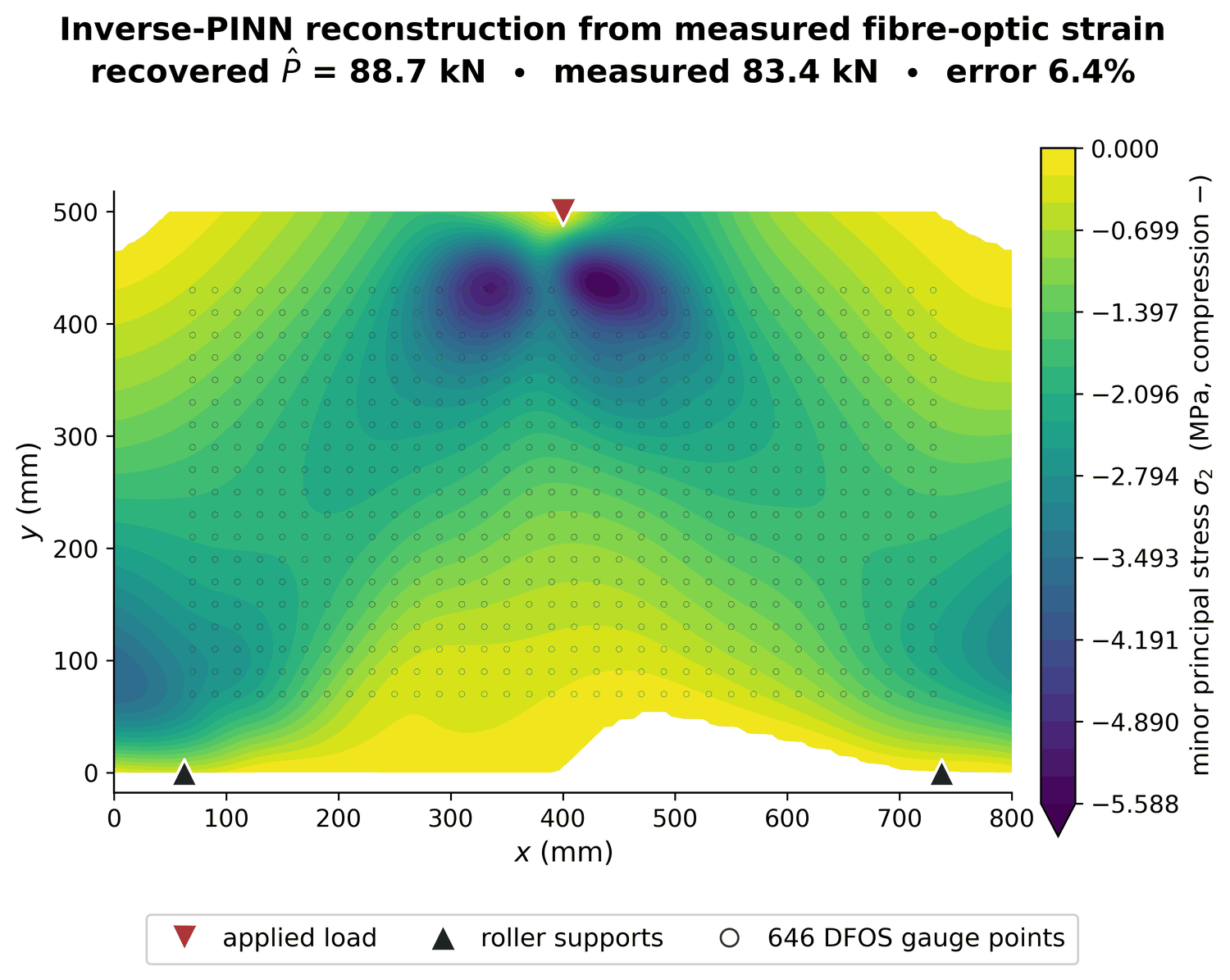
| Real fibre-optic wall, 646 measured points | no reference stress field | within 6.4% |
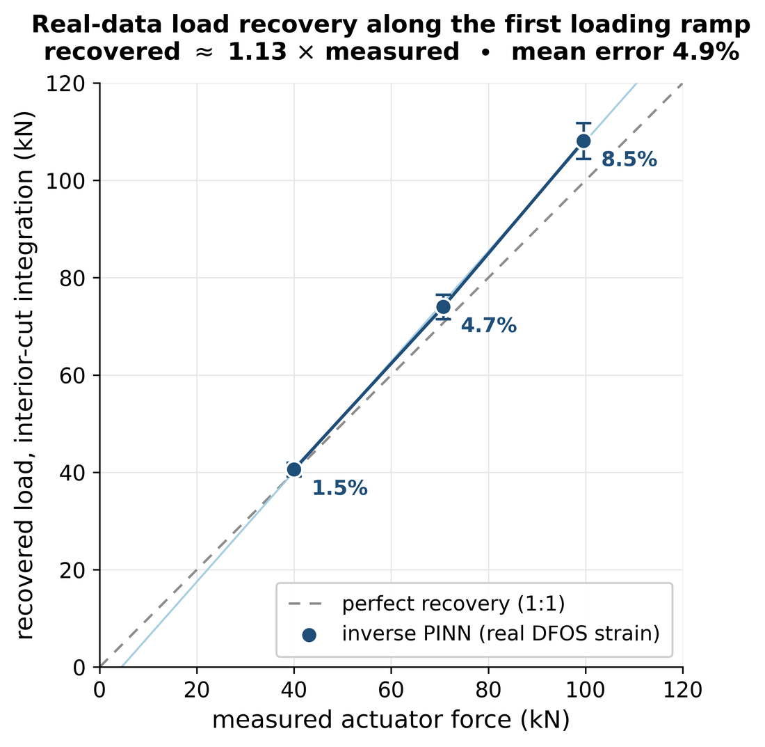
The last row is the one that matters most. Using the open distributed fibre-optic dataset of Fernandez and co-workers (2023), measured on a physical reinforced-concrete wall loaded as a D-region, the same network recovered the applied load as 88.7 kN against a measured 83.4 kN. Repeated along the loading history, the recovered load tracked the actuator force with errors between 1 and 9% and no systematic drift. The method works on genuine measured strain, not only on data produced by a solver.
A finding that reaches beyond this network
The study also isolates the mechanism that limits any strain-based CSFM assessment, whatever method is used to perform it.
In cracked concrete, the direction of the compression field follows the crack direction, and the crack direction is governed by the shear strain. So an error in measured shear strain rotates the whole compression field. We quantified it: a relative strain error propagates into the stress field amplified by a factor of about 3.4, a figure dominated by the shear strain component.
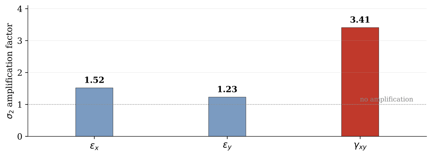
That gives engineers a practical rule: it tells you how accurate, and how dense, a strain measurement must be before a stress check built on it can be trusted. With a dense field at noise up to about 1%, the reconstruction stays below 10% error. At 3% gauge noise on the deep beam it grows to about 19%, just as the amplification predicts. That is a design input for any sensor layout on a D-region, whether or not a neural network is involved.
Two lessons for physics-informed machine learning
For readers who work with PINNs, two findings went against our first expectations:
- A forward, physics-only network was not competitive. Trained only against the governing equations, with no measurements, the network settled on diffuse, near-equilibrium fields far from the true one. The measurements are what make the problem well posed.
- The strong-form equilibrium residual hurt. Adding it as a training term degraded the field. Compatibility, the constitutive law and the traction conditions were sufficient. The reconstruction still satisfies equilibrium at the section level, because the stress integrated across any interior cut recovers the applied load.
Where this fits, and what it does not yet do
This is a step toward measurement-based assessment of existing concrete structures: strain from sensors in, a complete stress field and an estimate of the load out, with an explicit error bound attached. That is the kind of tool that load testing and structural health monitoring programs need to turn data into decisions.
It is also a first step, and the paper is clear about its limits. Apart from the real wall, the gauge data are synthetic. The cases are two-dimensional and plane-stress. The wall pier is checked at service load, about 41% of its tested ultimate capacity. An L-shaped geometry exposed a weakness of the current architecture that a domain-masked network should fix. Pile caps, hammerheads, dapped ends and the three-dimensional case, where the interior is genuinely hidden from surface sensors and the inverse framing is strongest, are the natural next steps.
In my bridge design work I check D-regions such as pier caps and pile caps with strut and tie models. That is much of why this question interested me: the design checks are well established, but reading the state of a D-region that is already in service is not.
If you would like to explore compatible stress fields interactively, my CSFM explorer runs in the browser.
Read the paper
S. Lamsal and R. Bhandari, “Inverse physics-informed neural network for CSFM stress field reconstruction in concrete D-regions,” Computer-Aided Civil and Infrastructure Engineering, vol. 50, art. 100192, 2026. DOI: 10.1016/j.cacaie.2026.100192
The article is open access under the Creative Commons Attribution 4.0 license, so it is free to read, share and adapt with attribution. The figures in this post are reproduced from it.
My thanks to my co-author, Rubi Bhandari of Florida International University, and to the editor and reviewers, whose comments led directly to the real-data validation.